CMU 10-414/714: Deep Learning Systems (2020) - 深度学习系统 04 Automatic Differentiation

Automatic Differentiation

1. hypothesis class: $x \rightarrow h_\theta(x)$, MLP
2. loss function(cross-entropy loss): $\ell(x, y) = -h_y(x) + \log \sum_{j=1}^n \exp(h_j(x))$
3. optimization method: $\theta := \theta - \alpha \nabla_\theta \ell$

机器学习/深度学习是否就是在学习参数集合 $\theta$?

除了 SGD 随机梯度下降，还有 Adam 等优化方法

计算 gradient 是一个很复杂的问题，但是现在有自动微分

Numerical differentiation

$$ \frac{\partial f(\theta)}{\partial \theta_i} = \lim_{\epsilon \to 0} \frac{f(\theta + \epsilon e_i) - f(\theta)}{\epsilon} \

\frac{\partial f(\theta)}{\partial \theta_i} \approx \frac{f(\theta + \epsilon e_i) - f(\theta - \epsilon e_i)}{2\epsilon} + o(\epsilon^2) $$

numerical error, less efficient to compute

一般用来做 checking？

Numerical gradient checking

$$\frac{\partial f(\theta)}{\partial \theta_i} \approx \frac{f(\theta + \epsilon \delta) - f(\theta - \epsilon \delta)}{2\epsilon}$$

检查 auto differentiation algo 是否正确

Symbolic differentiation

$$\frac{\partial (f(\theta) + g(\theta))}{\partial \theta} = \frac{\partial f}{\partial \theta} + \frac{\partial g}{\partial \theta}$$$$\frac{\partial (f(\theta) g(\theta))}{\partial \theta} = g(\theta) \frac{\partial f}{\partial \theta} + f(\theta) \frac{\partial g}{\partial \theta}$$$$\frac{\partial f(g(\theta))}{\partial \theta} = \frac{\partial f(g)}{\partial g(\theta)} \cdot \frac{\partial g(\theta)}{\partial \theta}$$

回顾偏微分法则

wasted computation:

$$f(\theta) = \prod_{i=1}^n \theta_i$$

为了避免冗余，现代机器学习和计算工具使用了自动微分（Automatic Differentiation）

这个函数求偏导，会有很多重复的乘积，可以用自动微分和计算图缓存中间结果

Computational graph

$$y = \ln(x_1) + x_1 \cdot x_2 - \sin(x_2)$$

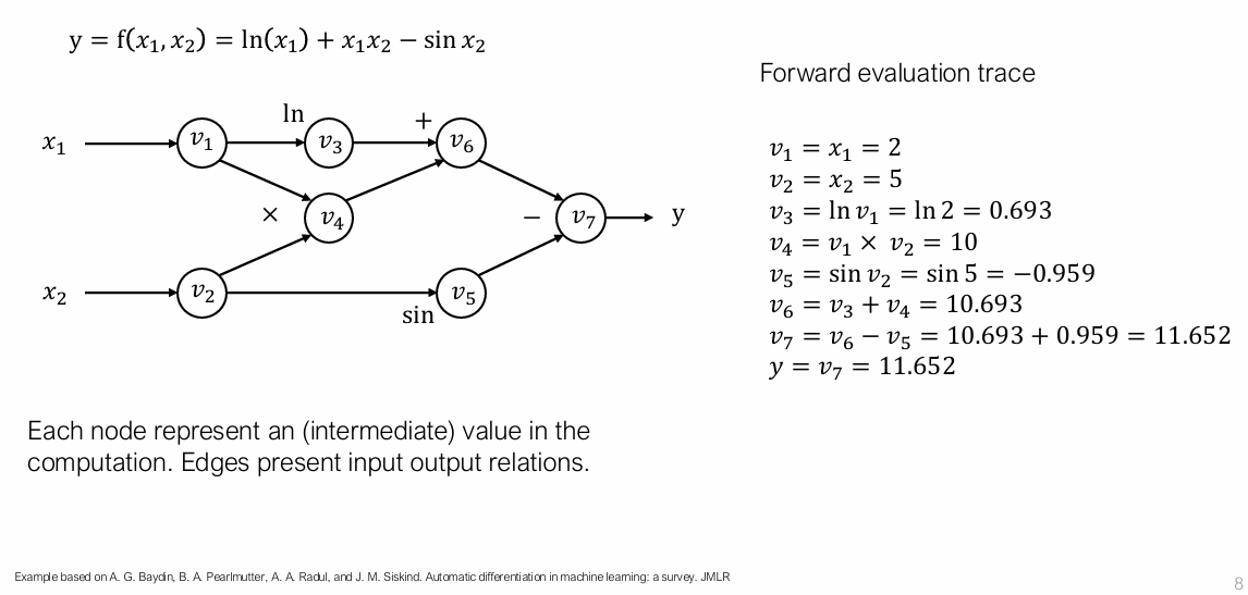
中间结果

Forward mode automatic differentiation (AD)

it automatically propagates gradients through a computational graph based on the mathematical operations involved.

不需要手动计算梯度 计算了很多中间值

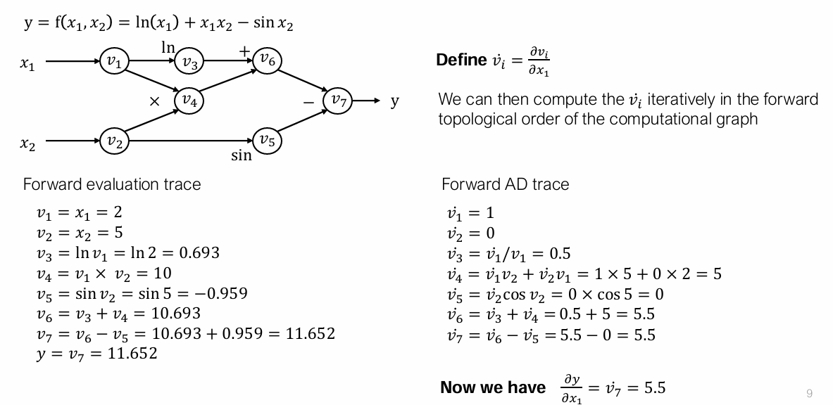
Limitation of forward mode AD

对于函数 $f: \mathbb{R}^n \to \mathbb{R}^k$ ，前向模式自动微分需要 n 次传递 来计算输出对所有 n 个输入变量的梯度。

也就是说，对于每个输入变量 $(x_1, x_2, \ldots, x_n )$，需要单独进行一次计算，以追踪输出随着该输入的变化。

在大多数情况下，当 $k = 1$ （标量输出，例如机器学习中的损失函数）且 $n$ 很大时（如神经网络的权重数量庞大），前向模式会显得 计算成本较高且效率低下，因为它的计算成本随着输入数量 $n$ 的增加线性增长。

We mostly care about the cases where $k = 1$ and large $n$ .

In order to resolve the problem efficiently, we need to use another kind of AD

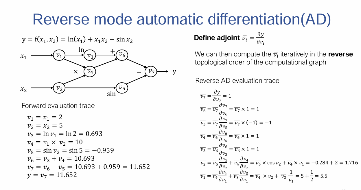
Reverse mode automatic differentiation(AD)

Adjoint: $\bar{v}_i = \frac{\partial y}{\partial v_i}$

每个变量的导数，但是反向计算

Reverse Mode 一次反向传递即可计算出 标量输出对所有输入的梯度，适用于 $f: \mathbb{R}^n \to \mathbb{R}^1$ 的情况（例如机器学习中的损失函数）。

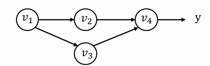
Derivation for the multiple pathway case

multiple pathways

$$ v_1 \

y = f(v_2, v_3) \

\frac{\partial y}{\partial v_1} = \frac{\partial f(v_2, v_3)}{\partial v_2} \cdot \frac{\partial v_2}{\partial v_1} + \frac{\partial f(v_2, v_3)}{\partial v_3} \cdot \frac{\partial v_3}{\partial v_1} $$

partial adjoint: $v_i \rightarrow v_j = \bar{v}_j \cdot \frac{\partial v_j}{\partial v_i}$

$$\bar{v}_i = \sum_{j \in \text{next}(i)} v_i \rightarrow v_j$$

We can compute partial adjoints separately then sum them together

自动微分（automatic differentiation）的背景下，针对多路径计算场景的偏导数的推导

用于表示 Reverse AD 算法

Reverse AD algorithm

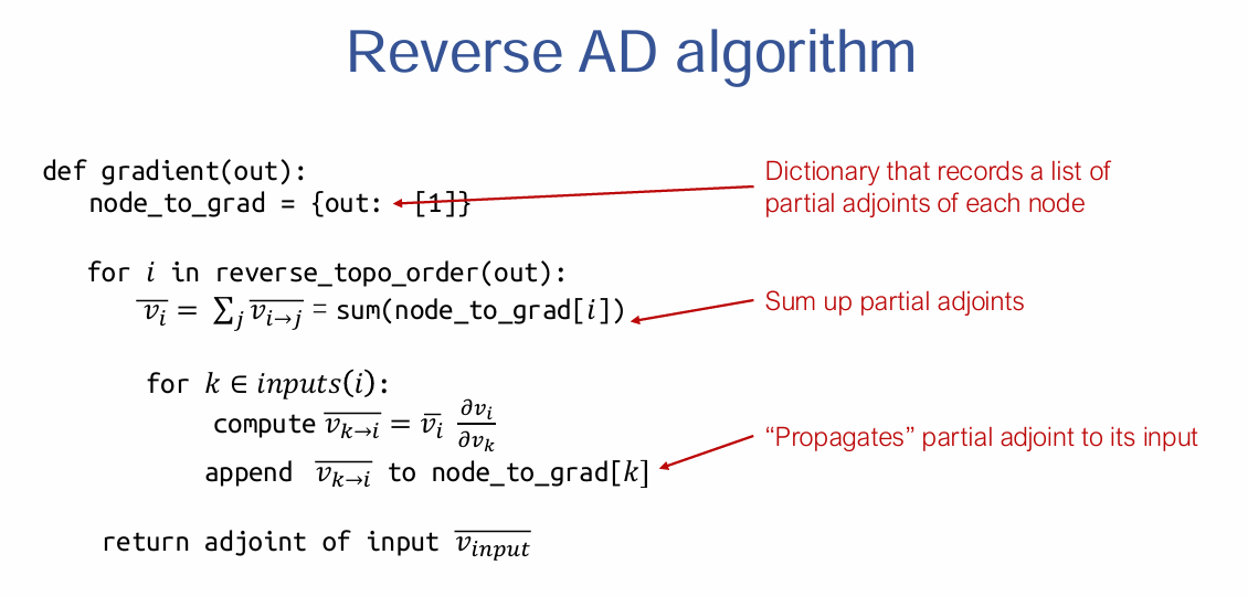
node_to_grad 记录 partial adjoint 用于缓存

Reverse mode AD by extending computational graph

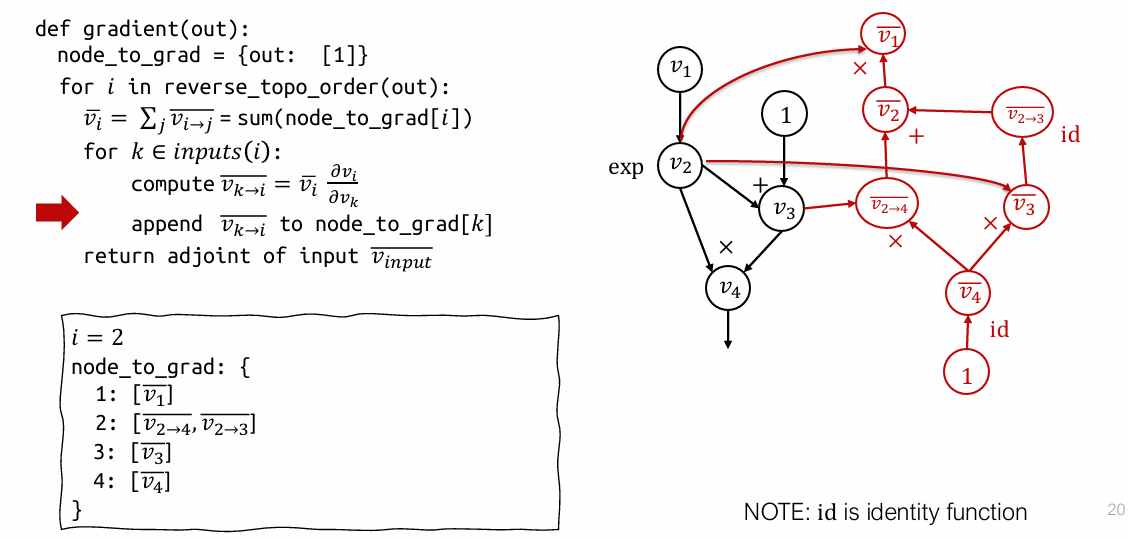
computational graph 拓展

Reverse mode AD vs Backprop

Backprop

• Run backward operations the same forward graph
• Used in first generation deep learning frameworks (caffe, cuda-convnet)

Reverse mode AD by extending computational graph

• Construct separate graph nodes for adjoints
• Used by modern deep learning frameworks

所以 reverse mode AD 自动微分就是缓存了一些其中的结果，用 adjoints 来表示

每次计算就不需要完全重新计算梯度、扩展的图

Reverse mode AD on Tensors

Define adjoint for tensor values

$$\bar{Z} = \frac{\partial y}{\partial Z} = \begin{bmatrix} \frac{\partial y}{\partial Z_{1,1}} & \cdots & \frac{\partial y}{\partial Z_{1,n}} \\ \vdots & \ddots & \vdots \\ \frac{\partial y}{\partial Z_{m,1}} & \cdots & \frac{\partial y}{\partial Z_{m,n}} \end{bmatrix}$$

Tensor 计算，reverse mode AD 的向量表达

下一张将讨论实现

pros/cons of backprop and reverse mode AD:

Handling gradient of gradient

The result of reverse mode AD is still a computational graph

We can extend that graph further by composing more operations and run reverse mode AD again on the gradient

Reverse mode AD on data structures

Key take away: Define “adjoint value” usually in the same data type as the forward value and adjoint propagation rule. Then the sample algorithm works